Assess Normality • MetaPipe

library(MetaPipe)

MetaPipe assesses the normality of variables (traits) by performing a Shapiro-Wilk test on the raw data (see Load Raw Data and Replace Missing Data). Based on whether or not the data approximates a normal distribution, an array of transformations will be computed, and the normality assessed one more time.

The diagram below shows the tree of transformations that can be performed, the user can specify the transformation values passing a vector with the argument transf_vals to the function assess_normality; by default, [2, e, 3, 4, 5, 6, 7, 8, 9, 10].

The function call is as follows:

assess_normality(raw_data = raw_data, 
                 excluded_columns = c(2, 3, ..., M), 
                 # Optional
                 cpus = 1, 
                 out_prefix = "metapipe", 
                 plots_dir = tempdir(), 
                 transf_vals = c(2, exp(1), 3, 4, 5, 6, 7, 8, 9, 10),
                 alpha = 0.05,
                 pareto_scaling = FALSE,
                 show_stats = TRUE)

where raw_data is a data frame containing the raw data, as described in Load Raw Data and excluded_columns is a vector containing the indices of the properties, e.g. c(2, 3, ..., M). The other arguments are optional, cpus is the number of cores to use, in other words, the number of concurrent traits to process, out_prefix is the prefix for output files, plots_dir is the output directory where the plots will be stored, and transf_vals is a vector containing the transformation values to be used when transforming the original data.

Example

The following histogram shows a sample data obtained from a normal distribution with the command rnorm, but it was transformed using the power (base 2) function; thus, the data seems to be skewed:

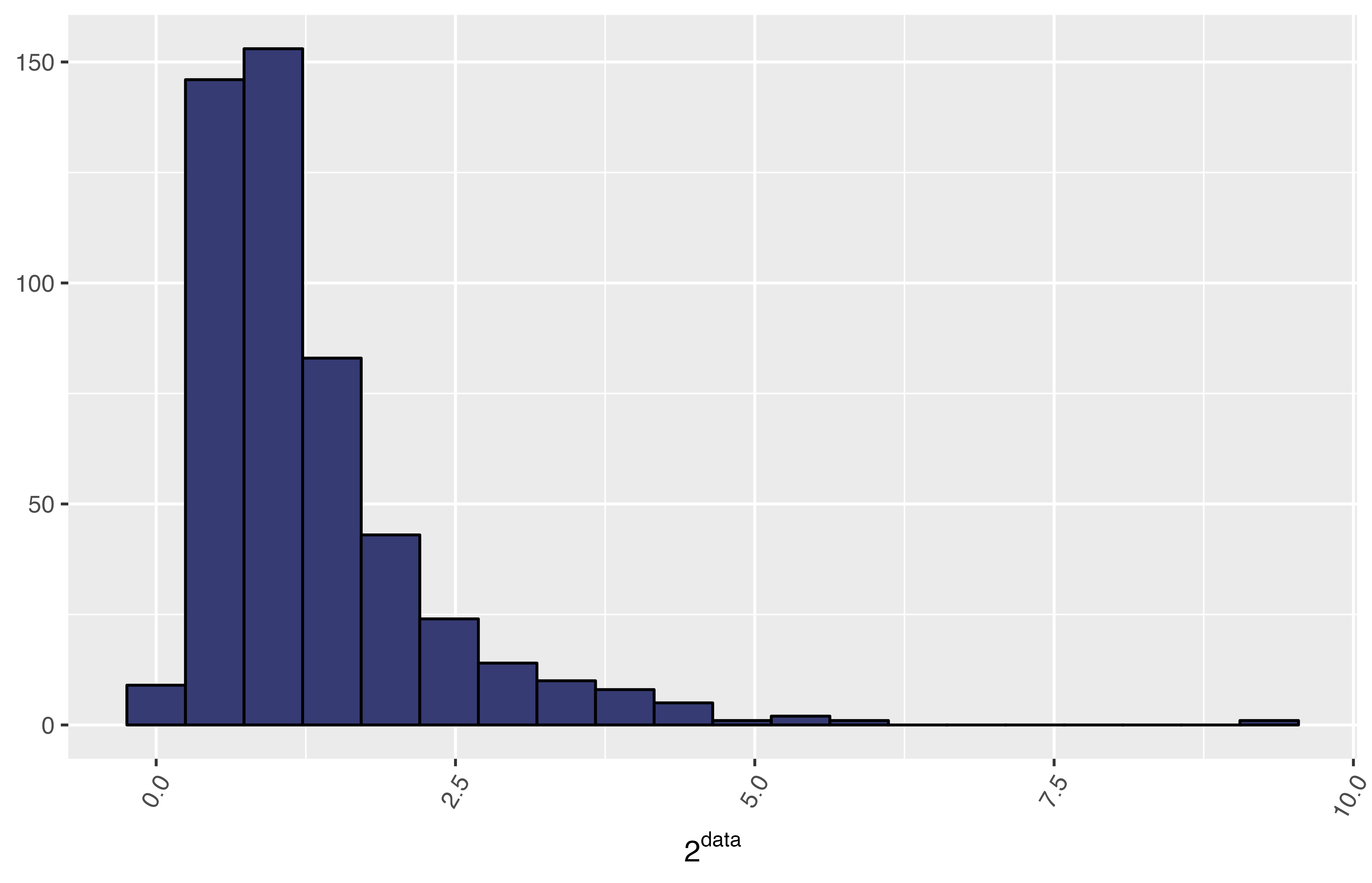
Using MetaPipe we can find an optimal transformation that “normalises” this data set:

example_data <- data.frame(ID = 1:500,
                           T1 = test_data,
                           T2 = 2^test_data)
workdir <- tempdir()
out_prefix <- file.path(workdir, "metapipe")
plots_dir <- workdir
normalised_data <- MetaPipe::assess_normality(example_data, c(1), 
                                              out_prefix = out_prefix, 
                                              plots_dir = plots_dir)
#> Total traits (excluding all NAs traits):     2
#> Normal traits (without transformation):      1
#> Normal traits (transformed):                 1
#> Total normal traits:                         2
#> Total skewed traits:                         0
#> 
#> Transformations' summary:
#>  f(x)      Value     # traits  
#>  log       2         1

normalised_data_norm <- normalised_data$norm
normalised_data_skew <- normalised_data$skew

transformed_data <- read.csv(file.path(workdir, 
                                       "metapipe_raw_data_normalised_all.csv"))

The output of this function is a long table of each trait, with the following format:

index	trait	values	flag	transf	transf_val

where index is a simple numeric value to uniquely identify each trait, trait is the trait/variable name, values is the actual entry, flag indicates whether the entry is parametric (Normal) or skewed (Non-normal), transf is the transformation function (empty for untransformed traits), and transf_val is the transformation value used.

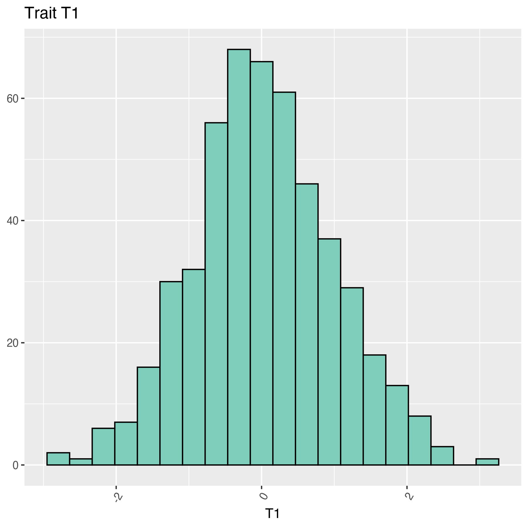
From the previous example, the top 5 entries for the trait T1 are:

index	trait	values	flag
1	T1	-0.5604756	Normal
1	T1	-0.2301775	Normal
1	T1	1.5587083	Normal
1	T1	0.0705084	Normal
1	T1	0.1292877	Normal
1	T1	1.7150650	Normal

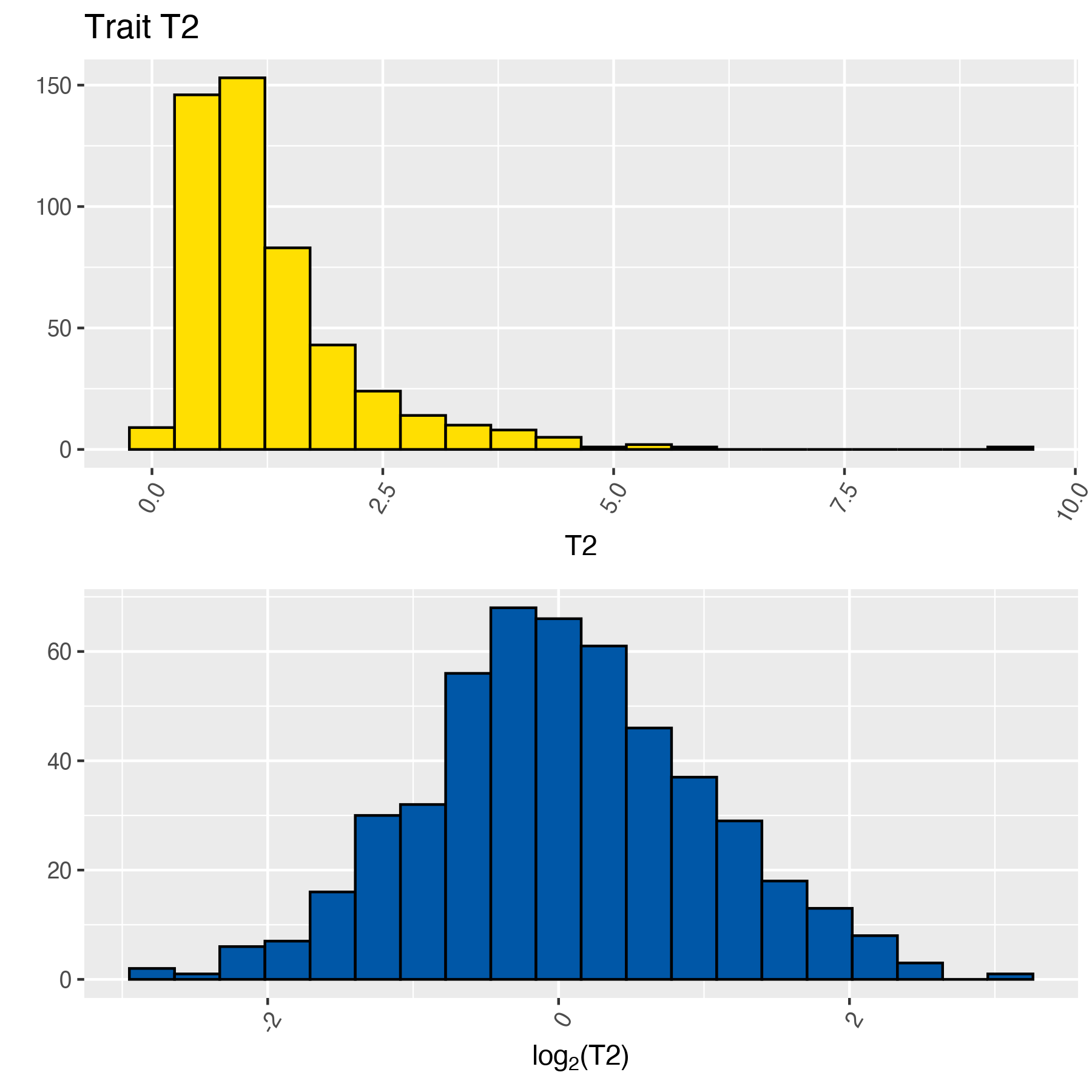
And for trait T2:

index	trait	values	flag	transf	transf_val
2	T2	-0.5604756	Normal	log	2
2	T2	-0.2301775	Normal	log	2
2	T2	1.5587083	Normal	log	2
2	T2	0.0705084	Normal	log	2
2	T2	0.1292877	Normal	log	2
2	T2	1.7150650	Normal	log	2

As expected both tables show the same entries; however, the latter indicates that T2 was transformed using \(\log_2\). The function will generate histograms for all the traits, the naming convention used is:

HIST_[index]_[transf]_[transf_val]_[trait].png for transformed traits
HIST_[index]_NORM_[trait].png for those that were not transformed.

For the previous data set HIST_1_NORM_T1.png and HIST_2_LOG_2_T2.png: